Generic Microprocessor Architectures for Cryptography

An application such as a set-top box can communicate with other media devices around the home. For example, it can download content to an iPod, interact with the home PC, or have an internet connection. These involve communication over different medium using different security protocols. In such security protocols, cryptography requires very intensive arithmetic which is time consuming for an embedded processor that typically has to respond to many interrupts from other functional blocks within the STB SoC. Our research investigates adaptable processor architectures that can be used to provide a means to offload the intensive arithmetic. Recent work in this area has included the design of two suitable architectures to support public and private key algorithms.

Adaptable, Scalable Public Key Cryptographic Processor Architecture

• Supports integer and polynomial arithmetic & optimised instructions that provide efficient field multiplication, addition and inversion
• Support of algorithms which include modular exponentiation (RSA), ECC over prime fields & ECC over binary fields
• Field & operand lengths only restricted by data RAM provided
  (previous designs have fixed field lengths)

Private Key RISC Microprocessor Architecture

Includes:

• Algorithm specific instructions: eg. GF Multiplication
• An extended Instruction set: common algorithm Bit-oriented & Byte-oriented instructions
• Co-processors of common algorithms eg. AES and DES
• 
• Private Key RISC Microprocessor Architecture

Intel 8085

The Intel 8085 is an 8-bit microprocessor introduced by Intel in 1977. It was binary-compatible with the more-famous Intel 8080 but required less supporting hardware, thus allowing simpler and less expensive microcomputer systems to be built.

The "5" in the model number came from the fact that the 8085 requires only a +5-volt (V) power supply rather than the +5V, -5V and +12V supplies the 8080 needed. Both processors were sometimes used in computers running the CP/M operating system, and the 8085 later saw use as a microcontroller, by virtue of its low component count. Both designs were eclipsed for desktop computers by the compatible Zilog Z80, which took over most of the CP/M computer market as well as taking a share of the booming home computer market in the early-to-mid-1980s.

An Intel 8085AH processor.
Produced	From 1977 to 1990s
Common manufacturer(s)	Intel and several others
Max. CPU clock rate	3,5 and 6 MHz
Instruction set	pre x86
Package(s)	40 pin DIP

The 8085 had a long life as a controller. Once designed into such products as the DECtape controller and the VT100 video terminal in the late 1970s, it continued to serve for new production throughout the life span of those products (generally longer than the product life of desktop computers).

Description


The 8085 is a conventional von Neumann design based on the Intel 8080. Unlike the 8080 it does not multiplex state signals onto the data bus, but the 8-bit data bus was instead multiplexed with the lower part of the 16-bit address bus to limit the number of pins to 40. Pin #40 is used for the power supply (+5v) and pin #20 for ground. Pin #39 is used as the hold pin. Pins #15 to #8 are generally used for address buses. The processor was designed using nMOS circuitry and the later "H" versions were implemented in Intel's enhanced nMOS process called HMOS, originally developed for fast static RAM products. Only a 5 Volt supply is needed, like competing processors and unlike the 8080. The 8085 uses approximately 6,500 transistors.[1]

The 8085 incorporates the functions of the 8224 (clock generator) and the 8228 (system controller), increasing the level of integration. A downside compared to similar contemporary designs (such as the Z80) was the fact that the buses required demultiplexing; however, address latches in the Intel 8155, 8355, and 8755 memory chips allowed a direct interface, so an 8085 along with these chips was almost a complete system.

The 8085 has extensions to support new interrupts, with three maskable interrupts (RST 7.5, RST 6.5 and RST 5.5), one non-maskable interrupt (TRAP), and one externally serviced interrupt (INTR). The RST n.5 interrupts refer to actual pins on the processor, a feature which permitted simple systems to avoid the cost of a separate interrupt controller.

i8085 microarchitecture.

Like the 8080, the 8085 can accommodate slower memories through externally generated wait states (pin 35, READY), and has provisions for Direct Memory Access (DMA) using HOLD and HLDA signals (pins 39 and 38). An improvement over the 8080 was that the 8085 can itself drive a piezoelectric crystal directly connected to it, and a built in clock generator generates the internal high amplitude two-phase clock signals at half the crystal frequency (a 6.14 MHz crystal would yield a 3.07 MHz clock, for instance).

Programming model

The 8085 is a binary compatible follow up on the 8080, using the same basic instruction set as the 8008 (developed by Computer Terminal Corporation). Only a few minor instructions were new to the 8085 above the 8080 set.

Registers

The processor has seven 8-bit registers named A, B, C, D, E, H, and L, where A is the 8-bit accumulator and the other six can be used as independent byte-registers or as three 16-bit register pairs, BC, DE, and HL, depending on the particular instruction. Some instructions use HL as a (limited) 16-bit accumulator. As in the 8080, the contents of the memory address pointed to by HL could be accessed as pseudoregister M. It also has a 16-bit stack pointer to memory (replacing the 8008's internal stack), and a 16-bit program counter. HL pair is called the primary data pointers.

Commands/instructions

As in many other 8-bit processors, all instructions are encoded in a single byte (including register-numbers, but excluding immediate data), for simplicity. Some of them are followed by one or two bytes of data, which could be an immediate operand, a memory address, or a port number. Like larger processors, it has CALL and RET instructions for multi-level procedure calls and returns (which can be conditionally executed, like jumps) and instructions to save and restore any 16-bit register-pair on the machine stack. There are also eight one-byte call instructions (RST) for subroutines located at the fixed addresses 00h, 08h, 10h,...,38h. These were intended to be supplied by external hardware in order to invoke a corresponding interrupt-service routine, but are also often employed as fast system calls. The most sophisticated command was XTHL, which is used for exchanging the register pair HL with the value stored at the address indicated by the stack pointer.

8-bit instructions

Most 8-bit operations work on the 8-bit accumulator (the A register). For two operand 8-bit operations, the other operand can be either an immediate value, another 8-bit register, or a memory cell addressed by the 16-bit register pair HL. Direct copying is supported between any two 8-bit registers and between any 8-bit register and a HL-addressed memory cell. Due to the regular encoding of the MOV-instruction (using a quarter of available opcode space) there are redundant codes to copy a register into itself (MOV B,B, for instance), which are of little use, except for delays. However, what would have been a copy from the HL-addressed cell into itself (i.e., MOV M,M) instead encodes the HLT instruction, halting execution until an external reset or interrupt occurred.

16-bit operations

Although the 8085 is an 8-bit processor, it also has some 16-bit operations. Any of the three 16-bit register pairs (BC, DE, HL) or SP could be loaded with an immediate 16-bit value (using LXI), incremented or decremented (using INX and DCX), or added to HL (using DAD). LHLD loaded HL from directly-addressed memory and SHLD stored HL likewise. The XCHG operation exchanges the values of HL and DE. Adding HL to itself performs a 16-bit arithmetical left shift with one instruction. The only 16 bit instruction that affects any flag was DAD (adding HL to BC, DE, HL or SP), which updates the carry flag to facilitate 24-bit or larger additions and left shifts (for a floating point mantissa for instance). Adding the stack pointer to HL is useful for indexing variables in (recursive) stack frames. A stack frame can be allocated using DAD SP and SPHL, and a branch to a computed pointer can be done with PCHL. These abilities make it feasible to compile languages such as PL/M, Pascal, or C with 16-bit variables and produce 8085 machine code.

Subtraction and bitwise logical operations on 16 bits is done in 8-bit steps. Operations that have to be implemented by program code (subroutine libraries) included comparisons of signed integers as well as multiply and divide.

Input/output scheme

The 8085 supported up to 256 input/output (I/O) ports, accessed via dedicated I/O instructions—taking port addresses as operands. This I/O mapping scheme was regarded as an advantage, as it freed up the processor's limited address space. Many CPU architectures instead use a common address space without the need for dedicated I/O instructions, although a drawback in such designs may be that special hardware must be used to insert wait states as peripherals are often slower than memory. However, in some simple 8080 computers, I/O was indeed addressed as if they were memory cells, "memory mapped", leaving the I/O commands unused. I/O addressing could also sometimes employ the fact that the processor would output the same 8-bit port address to both the lower and the higher address byte (i.e. IN 05h would put the address 0505h on the 16-bit address bus). Similar I/O-port schemes are used in the 8080-compatible Zilog Z80 as well as the closely related x86 families of microprocessors.

Development system

Intel produced a series of development systems for the 8080 and 8085, known as the MDS-80 Microprocessor System. The original development system had an 8080 processor. Later 8085 and 8086 support was added including ICE (in-circuit emulators). It was a large and heavy desktop box, about a 20" cube (in the Intel corporate blue colour) which included a CPU, monitor, and a single 8 inch floppy disk drive. Later an external box was available with two more floppy drives. It ran the ISIS operating system and could also operate an emulator pod and an external EPROM programmer. This unit used the Multibus card cage which was intended just for the development system. A surprising number of spare card cages and processors were being sold, leading to the development of the Multibus as a separate product.

The later iPDS was a portable unit, about 8" x 16" x 20", with a handle. It had a small green screen, a keyboard built into the top, a 5¼ inch floppy disk drive, and ran the ISIS-II operating system. It could also accept a second 8085 processor, allowing a limited form of multi-processor operation where both processors ran simultaneously and independently. The screen and keyboard could be switched between them, allowing programs to be assembled on one processor (large programs took awhile) while files were edited in the other. It had a bubble memory option and various programming modules, including EPROM and Intel 8048 and 8051 programming modules which were plugged into the side, replacing stand-alone device programmers. In addition to an 8080/8085 assembler, Intel produced a number of compilers including PL/M-80 and Pascal languages, and a set of tools for linking and statically locating programs to enable them to be burnt into EPROMs and used in embedded systems. The hardware support changes were announced and supported, but the software upgrades were not supported by the assembler, user manual or any other means. At times it was claimed they were not tested when that was false.

Applications

For the extensive use of 8085 in various applications, the microprocessor is provided with an instruction set which consists of various instructions such as MOV, ADD, SUB, JMP etc. These instructions are written in the form of a program which is used to perform various operations such as branching, addition, subtraction, bitwise logical and bit shift operations. More complex operations and other arithmetic operations must be implemented in software. For example, multiplication is implemented using a multiplication algorithm.

The 8085 processor has found marginal use in small scale computers up to the 21st century. The TRS-80 Model 100 line uses a 80C85. The CMOS version 80C85 of the NMOS/HMOS 8085 processor has several manufacturers, and some versions (eg. Tundra Semiconductor Corporation's CA80C85B) have additional functionality, eg. extra machine code instructions. One niche application for the rad-hard version of the 8085 has been in on-board instrument data processors for several NASA and ESA space physics missions in the 1990s and early 2000s, including CRRES, Polar, FAST, Cluster, HESSI, the Sojourner Mar Rover , and THEMIS. The Swiss company SAIA used the 8085 and the 8085-2 as the CPUs of their PCA1 line of programmable logic controllers during the 1980s.

MCS-85 Family

The 8085 CPU was only one part of a much larger family of chips developed by Intel, for building a complete system. Although the 8085 CPU itself was not a great success, many of these support chips (or their descendents) later found their use in combination with the 8086 microprocessor. For example, the original IBM PC based on the Intel 8088 processor used many of these chips, and the prominence of IBM PC compatibles is why many of these chips are still in use today, although not as the chips themselves, but with their equivalent functionality embedded into larger VLSI chips, namely the "Southbridge" chips of modern PCs.

* 8007-Ram controller
* 8085-CPU
* 8155-RAM+ 3 I/O Ports+Timer
* 8156-RAM+ 3 I/O Ports+Timer
* 8185-SRAM
* 8202-Dynamic RAM Controller
* 8203-Dynamic RAM Controller
* 8205-1 Of 8 Binary Decoder
* 8206-Error Detection & Correction Unit
* 8207-DRAM Controller
* 8210-TTL To MOS Shifter & High Voltage Clock Driver
* 8212-8 Bit I/O Port
* 8216-4 Bit Parallel Bidirectional Bus Driver
* 8218/8219-Bus Controller
* 8222-Dynamic RAM Refresh Controller
* 8226-4 Bit Parallel Bidirectional Bus Driver
* 8231-Arithmetic Processing Unit
* 8232-Floating Point Processor
* 8237-DMA Controller
* 8251-Communication Controller
* 8253-Programmable Interval Timer
* 8254-Programmable Interval Timer
* 8255-Programmable Peripheral Interface
* 8256-Multifunction Support Controller
* 8257-DMA Controller
* 8259-Programmable Interrupt Controller
* 8271-Programmable Floppy Disk Controller
* 8272-Single/Double Density Floppy Disk Controller
* 8273-Programmable HDLC/SDLC Protocol Controller
* 8274-Multi-Protocol Serial Controller
* 8275-CRT Controller
* 8276-Small System CRT Controller
* 8278-Programmable Key Board Interface
* 8279-Key Board/Display Controller
* 8282-8-bit Non-Inverting Latch with Output Buffer
* 8283-8-bit Inverting Latch with Output Buffer
* 8291-GPIB Talker/Listener
* 8292-GPIB Controller
* 8293-GPIB Transceiver
* 8294-Data Encryption/Decryption Unit+1 O/P Port
* 8295-Dot Matrix Printer Controller
* 8296-GPIB Transceiver
* 8297-GPIB Transceiver
* 8355-16,384-bit (2048 x 8) ROM with I/O
* 8604-4096-bit (512 x 8) PROM
* 8702-2K-bit (265 x 8 ) PROM
* 8755-EPROM+2 I/O Ports

Motorola 6800

Motorola MC6800 Microprocessor.

The 6800 was an 8-bit microprocessor designed and manufactured by Motorola in 1974. The MC6800 microprocessor was part of the M6800 Microcomputer System that also included serial and parallel interface ICs, RAM, ROM and other support chips. A significant design feature was that the M6800 family of ICs required only a single five-volt power supply; other microprocessors required three voltages. The M6800 Microcomputer System was announced in March 1974 and was in full production by the end of that year.The 6800 architecture and instruction set were influenced by the then popular Digital Equipment Corporation PDP-11 mini computer.The 6800 had a 16-bit address bus address that could access 64 KB of memory and a 8-bit bi-directional data bus. It has 72 instructions with seven addressing modes for a total of 192 opcodes. The original MC6800 could have a clock rate of up to 1 MHz. Later versions had a maximum clock rate of 2 MHz.In addition to the ICs, Motorola also provided a complete assembly language development system. The customer could use the software on a remote timeshare computer or on an in-house mini-computer system. The Motorola EXORciser was a desktop computer built with the M6800 ICs that could be used for prototyping and debugging new designs. An expansive documentation package included datasheets on all ICs, two assembly language programming manuals, and a 700 page application manual that showed how to design a point-of-sale computer terminal.The 6800 was popular in computer peripherals, test equipment applications and point-of-sale terminals. The MC6802, introduced in 1977, included 128 byte of RAM and an internal clock oscillator on chip. The MC6801 and MC6805 included with RAM, ROM and I/O on a single chip were popular in automotive applications.

Motorola's history in semiconductors

Motorola transistor radio, 1960.

Galvin Manufacturing Corporation was founded in 1928 in Chicago, Illinois and produced their first Motorola brand car radio in 1930. The company name was changed to Motorola in 1947. A research and development center was opened in Phoenix, Arizona in 1949 and they began commercial production of transistors at a new $1.5 million facility in Phoenix in 1955. In 1966 an integrated circuit facility was built in the Phoenix suburb of Mesa.In 1973, they announced plans to build a new plant in Austin, Texas to manufacture MOS integrated circuits. The microprocessor group moved from Mesa to Austin in 1975.Motorola's transistors and integrated circuits were used in-house for their communication, military, automotive and consumer products and they were also sold to other companies. In the 1960s, Motorola sold a full line of digital ICs that were used in computers, test equipment and industrial controls. By 1970 they were producing metal-oxide semiconductors (MOS) LSI chips as standard products and custom circuits. They also produced semiconductor memories that were used in calculators, point-of-sale terminals and computers. Motorola's sales had reached $1.2 billon in 1973 and they had 64,000 employees. The Semiconductor Products Division (SPD) had sales of $419 million and was the second largest semiconductor company after Texas Instruments.Intel was founded in 1968 and had sales of $66 million in 1973.In the early 1970s Motorola started a project that developed their first microprocessor, the MC6800. This was followed by single chip microcontrollers such as the MC6801 and MC6805. In 1979 the 16-bit version of MC68000 microprocessor was introduced, this processor was later extended to 32 bits.
In 1999 Motorola spun off their analog IC, digital IC and transistor business to ON Semiconductor of Phoenix Arizona. In 2004 they spun off their microprocessor business to Freescale Semiconductor of Austin, Texas.

Development team

Motorola did not chronicle the development of the 6800 microprocessor the way that Intel did for their microprocessors. In 2008 the Computer History Museum interviewed four members of the 6800 microprocessor design team. Their recollections can be confirmed and expanded by magazine and journal articles written at the time.

The Motorola microprocessor project began in 1971 with a team composed of designer Tom Bennett, engineering director Jeff LaVell, product marketer Link Young and systems designers Mike Wiles, Gene Schriber and Doug Powell. They were all located in Mesa, Arizona. By the time the project was finished, Bennett had 17 chip designers and layout people working on five chips. LaVell had 15 to 20 system engineers and there was another applications engineering group of similar size.

Tom Bennett had a background in industrial controls and had worked for Victor Comptometer in the 1960s designing the first electronic calculator to use MOS ICs, the Victor 3900. In May 1969 Ted Hoff showed Bennett early diagrams of the Intel 4004 to see if it would meet their calculator needs. Bennett joined Motorola in 1971 to design calculator ICs. He was soon assigned as the chief architect of the microprocessor project that produced the 6800. Others have taken credit for designing the 6800. In September 1975 Robert Cushman, EDN magazine's microprocessor editor, interviewed Chuck Peddle about MOS Technology's new 6502 microprocessor. Cushman then asked "Tom Bennett, master architect of the 6800," to comment about this new competitor. After the 6800 project Bennett worked on automotive applications and Motorola became a major supplier of microprocessors used in automobiles.

Jeff LaVell joined Motorola in 1966 and worked in the computer industry marketing organization. Jeff had previously worked for Collins Radio on their C8500 computer that was built with small scale ECL ICs. In 1971 he led a group that examined the needs of their existing customers such as: Hewlett Packard, National Cash Register, National Data Corporation (CDC), and Digital Equipment Corporation. They would study the customer's products and tried to identify functions that could be implemented in larger integrated circuits at a lower cost. The result of the survey was a family of 15 building bocks; each could be implemented in an integrated circuit. Some of these blocks were implemented in the initial M6800 release and more were added over the next few years. To evaluate the 6800 architecture while the chip was being designed, Jeff's team built an equivalent circuit using 451 small scale TTL ICs on five 10 by 10 inch (25 by 25 cm) circuit boards. Later they reduced this to 114 ICs on one board by using ROMs and MSI logic devices.

John Buchanan was a memory designer at Motorola when Bennett asked him to design a voltage doubler to for the 6800. Typical n-channel MOS IC's required three power supplies: -5 volts, +5 volts and +12 volts. The M6800 family was to use only one, +5 volts. It was easy to eliminate the -5 volt supply but the MOS transistors needed a supply of 10 to 12 volts. This on-chip voltage doubler would supply the higher voltage and Buchanan did the circuit design, analysis and layout for the 6800 microprocessor. He received patents on the voltage doubler and the 6800 chip layout. Rod Orgill assisted Buchanan with analyses and 6800 chip layout. Later Orgill would design the MOS Technology 6501 microprocessor that was socket compatible with the 6800.

Bill Lattin joined Motorola in 1969 and his group provided the computer simulation tools for characterizing the new MOS circuits in the 6800. Lattin and Frank Jenkins had both attended UC Berkley and studied computer circuit simulators under Donald Pederson, the designer of the SPICE circuit simulator. Motorola's simulator, MTIME, was an advanced version of the TIME circuit simulator that Jenkins had developed at Berkley. The group published a technical paper, "MOS-device modeling for computer implementation" in 1973 describing a "5-V single-supply n-channel technology" operating at 1 MHz. They could simulate a 50 MOSFET circuit on an IBM 370/165 mainframe computer. In November 1975, Lattin joined Intel to work on their next generation microprocessor.

Bill Mensch joined Motorola in 1971 after graduating from the University of Arizona. He had worked several years as an electronics technician before earning his BSEE degree. The first year at Motorola was a series of three month rotations through four different areas. Memsch did a flowchart for a modem that would become the 6860. He also worked the application group that was defining the M6800 system. After this training year, he was assigned to the 6820 Parallel Interface Adapter (PIA) development team. Mensch was a major contributor to the design of this chip and received a patent on the IC layout and was named as a co-inventor of seven other M6800 system patents. Later Mensch would design the MOS Technology 6502 microprocessor.

Mike Wiles was a design engineer in Jeff LaVell's group and made numerous customer visits with Tom Bennett during 6800 product definition phase. He is listed as an inventor on eighteen 6800 patents but is best known for a computer program, MIKBUG.This was a rudimentary BIOS for a 6800 computer system that allowed the user to examine the contents of RAM and to save or load programs to tape. This 512 byte program occupied half of a MCM6830 ROM. This ROM was used in the Motorola MEK6800 design evaluation kit and early hobby computer kits. Wiles stayed with Motorola, moved to Austin and helped design the MC6801 microcontroller that was released in 1978.

Chuck Peddle joined the design team in 1973 after the 6800 processor design was done but he contributed to overall system design and to several peripheral chips, particularly the 6820 (PIA) parallel interface. Peddle is listed as an inventor on sixteen Motorola patents, most have six or more co-inventors. Like the other engineers of the team, Peddle visited potential customers and solicited their feedback. Peddle and John Buchanan built one of the earliest 6800 demonstration boards. In August 1974 Chuck Peddle left Motorola and joined a small semiconductor company in Pennsylvania, MOS Technology. There he led the team that designed the 6500 microprocessor family.

MIKBUG was part of the extensive M6800 microcomputer support developed by Motorola's Application Engineering Group.

MC6800 microprocessor design

The Motorola 6800 and the Intel 8080 were designed at the same time and were similar in function. The 8080 was a superset of the Intel 8008 which was based on the Datapoint 2200 processor. The 6800 architecture was modeled after the DEC PDP-11 processor. Both are TTL compatible, have an 8-bit bidirectional data bus, a 16-bit stack pointer, a 16-bit address bus that can address 64 KB of memory and come in a 40-pin DIP package. The 6800 has two accumulators and a 16-bit index register. The Direct Addressing mode allows fast access the first 256 bytes of memory. I/O devices are addressed as memory so there are no special I/O instructions. The 8080 has more internal registers and instructions for dedicated I/O ports. When the 8080 was reset, the program counter was cleared and the processor started at memory location 0000. The 6800 loaded the program counter from the highest address and started at the memory location stored there. The 6800's has a three-state control that will disable the address bus to allow another device direct memory access. A disk controller could transfer data into memory with no load on the processor. It is even possible to have two 6800 processors access the same memory.

MOS ICs typically used dual clock signals (a two-phase clock) in the 1970s. These were generated externally for both the 6800 and the 8080. The next generation of microprocessors incorporated the clock generation on chip. The 8080 had a 2 MHz clock but the processing throughput was similar to the 1 MHz 6800. The 8080 require more clock cycles to execute a processor instruction. The 6800 had a minimum clock rate of 100 kHz while the 8080 could be halted. Higher speed versions of both microprocessors were released by 1976.

A Motorola MC6800 microprocessor registers and I/O lines.

Other divisions in Motorola developed components for the M6800 family. The Components Products Department designed the MC6870 two-phase clock IC; the Memory Products group provided a full line of ROMs and RAMs. The CMOS group's MC14411 Bit Rate Generator provided a 75 to 9600 baud clock for the MC6850 serial interface. The buffers for address and data buses were standard Motorola products. Motorola could supply every IC, transistor and diode necessary to build a MC6800 based computer.

Basic principles of Transformer

The transformer is based on two principles: first, that an electric current can produce a magnetic field (electromagnetism), and, second that a changing magnetic field within a coil of wire induces a voltage across the ends of the coil (electromagnetic induction). Changing the current in the primary coil changes the magnetic flux that is developed. The changing magnetic flux induces a voltage in the secondary coil.An ideal transformer is shown in the adjacent figure. Current passing through the primary coil creates a magnetic field. The primary and secondary coils are wrapped around a core of very high magnetic permeability, such as iron, so that most of the magnetic flux passes through both the primary and secondary coils.

An ideal transformer

Induction law

The voltage induced across the secondary coil may be calculated from Faraday's law of induction, which states that:

where Vs is the instantaneous voltage, Ns is the number of turns in the secondary coil and Φ is the magnetic flux through one turn of the coil. If the turns of the coil are oriented perpendicular to the magnetic field lines, the flux is the product of the magnetic flux density B and the area A through which it cuts. The area is constant, being equal to the cross-sectional area of the transformer core, whereas the magnetic field varies with time according to the excitation of the primary. Since the same magnetic flux passes through both the primary and secondary coils in an ideal transformer, the instantaneous voltage across the primary winding equals

Taking the ratio of the two equations for V_s and V_p gives the basic equation for stepping up or stepping down the voltage

Ideal power equation

If the secondary coil is attached to a load that allows current to flow, electrical power is transmitted from the primary circuit to the secondary circuit. Ideally, the transformer is perfectly efficient; all the incoming energy is transformed from the primary circuit to the magnetic field and into the secondary circuit. If this condition is met, the incoming electric power must equal the outgoing power:

P_\text{incoming} = I_\text{p} V_\text{p} = P_\text{outgoing} = I_\text{s} V_\text{s},\!

giving the ideal transformer equation

\frac{V_\text{s}}{V_\text{p}} = \frac{N_\text{s}}{N_\text{p}} = \frac{I_\text{p}}{I_\text{s}}.

Transformers normally have high efficiency, so this formula is a reasonable approximation.

The ideal transformer as a circuit element

If the voltage is increased, then the current is decreased by the same factor. The impedance in one circuit is transformed by the square of the turns ratio. For example, if an impedance Zs is attached across the terminals of the secondary coil, it appears to the primary circuit to have an impedance of (Np/Ns)2Zs. This relationship is reciprocal, so that the impedance Zp of the primary circuit appears to the secondary to be (Ns/Np)2Zp.

Detailed operation

The simplified description above neglects several practical factors, in particular the primary current required to establish a magnetic field in the core, and the contribution to the field due to current in the secondary circuit.

Models of an ideal transformer typically assume a core of negligible reluctance with two windings of zero resistance. When a voltage is applied to the primary winding, a small current flows, driving flux around the magnetic circuit of the core. The current required to create the flux is termed the magnetizing current; since the ideal core has been assumed to have near-zero reluctance, the magnetizing current is negligible, although still required to create the magnetic field.

The changing magnetic field induces an electromotive force (EMF) across each winding. Since the ideal windings have no impedance, they have no associated voltage drop, and so the voltages VP and VS measured at the terminals of the transformer, are equal to the corresponding EMFs. The primary EMF, acting as it does in opposition to the primary voltage, is sometimes termed the "back EMF". This is due to Lenz's law which states that the induction of EMF would always be such that it will oppose development of any such change in magnetic field.

Practical considerations

Leakage flux

The ideal transformer model assumes that all flux generated by the primary winding links all the turns of every winding, including itself. In practice, some flux traverses paths that take it outside the windings. Such flux is termed leakage flux, and results in leakage inductance in series with the mutually coupled transformer windings. Leakage results in energy being alternately stored in and discharged from the magnetic fields with each cycle of the power supply. It is not directly a power loss (see "Stray losses" below), but results in inferior voltage regulation, causing the secondary voltage to fail to be directly proportional to the primary, particularly under heavy load. Transformers are therefore normally designed to have very low leakage inductance.

However, in some applications, leakage can be a desirable property, and long magnetic paths, air gaps, or magnetic bypass shunts may be deliberately introduced to a transformer's design to limit the short-circuit current it will supply. Leaky transformers may be used to supply loads that exhibit negative resistance, such as electric arcs, mercury vapor lamps, and neon signs; or for safely handling loads that become periodically short-circuited such as electric arc welders.

Air gaps are also used to keep a transformer from saturating, especially audio-frequency transformers in circuits that have a direct current flowing through the windings.[citation needed]

Leakage flux of a transformer

Leakage inductance is also helpful when transformers are operated in parallel. It can be shown that if the "per-unit" inductance of two transformers is the same (a typical value is 5%), they will automatically split power "correctly" (e.g. 500 kVA unit in parallel with 1,000 kVA unit, the larger one will carry twice the current).

Effect of frequency

The time-derivative term in Faraday's Law shows that the flux in the core is the integral with respect to time of the applied voltage.[36] Hypothetically an ideal transformer would work with direct-current excitation, with the core flux increasing linearly with time.[37] In practice, the flux would rise to the point where magnetic saturation of the core occurs, causing a huge increase in the magnetizing current and overheating the transformer. All practical transformers must therefore operate with alternating (or pulsed) current.

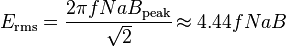
Transformer universal EMF equation

If the flux in the core is purely sinusoidal, the relationship for either winding between its rms voltage E_rms of the winding , and the supply frequency f, number of turns N, core cross-sectional area a and peak megnetic flux density B is given by the universal EMF equation:

If the flux does not contain even harmonics the following equation can be used for half-cycle average voltage E_avg of any waveshape:

The EMF of a transformer at a given flux density increases with frequency. By operating at higher frequencies, transformers can be physically more compact because a given core is able to transfer more power without reaching saturation and fewer turns are needed to achieve the same impedance. However, properties such as core loss and conductor skin effect also increase with frequency. Aircraft and military equipment employ 400 Hz power supplies which reduce core and winding weight. Conversely, frequencies used for some railway electrification systems were much lower (e.g. 16.7 Hz and 25 Hz) than normal utility frequencies (50 – 60 Hz) for historical reasons concerned mainly with the limitations of early electric traction motors. As such, the transformers used to step down the high over-head line voltages (e.g. 15 kV) are much heavier for the same power rating than those designed only for the higher frequencies.

Operation of a transformer at its designed voltage but at a higher frequency than intended will lead to reduced magnetizing current; at lower frequency, the magnetizing current will increase. Operation of a transformer at other than its design frequency may require assessment of voltages, losses, and cooling to establish if safe operation is practical. For example, transformers may need to be equipped with "volts per hertz" over-excitation relays to protect the transformer from overvoltage at higher than rated frequency.

One example of state-of-the-art design is those transformers used for electric multiple unit high speed trains, particularly those required to operate across the borders of countries using different standards of electrification. The position of such transformers is restricted to being hung below the passenger compartment. They have to function at different frequencies (down to 16.7 Hz) and voltages (up to 25 kV) whilst handling the enhanced power requirements needed for operating the trains at high speed.

Knowledge of natural frequencies of transformer windings is of importance for the determination of the transient response of the windings to impulse and switching surge voltages.

Energy losses

An ideal transformer would have no energy losses, and would be 100% efficient. In practical transformers energy is dissipated in the windings, core, and surrounding structures. Larger transformers are generally more efficient, and those rated for electricity distribution usually perform better than 98%.

Experimental transformers using superconducting windings achieve efficiencies of 99.85%. The increase in efficiency from about 98 to 99.85% can save considerable energy, and hence money, in a large heavily-loaded transformer; the trade-off is in the additional initial and running cost of the superconducting design.

Losses in transformers (excluding associated circuitry) vary with load current, and may be expressed as "no-load" or "full-load" loss. Winding resistance dominates load losses, whereas hysteresis and eddy currents losses contribute to over 99% of the no-load loss. The no-load loss can be significant, so that even an idle transformer constitutes a drain on the electrical supply and a running cost; designing transformers for lower loss requires a larger core, good-quality silicon steel, or even amorphous steel, for the core, and thicker wire, increasing initial cost, so that there is a trade-off between initial cost and running cost. (Also see energy efficient transformer).

Transformer losses are divided into losses in the windings, termed copper loss, and those in the magnetic circuit, termed iron loss. Losses in the transformer arise from:

Winding resistance

Current flowing through the windings causes resistive heating of the conductors. At higher frequencies, skin effect and proximity effect create additional winding resistance and losses.

Hysteresis losses

Each time the magnetic field is reversed, a small amount of energy is lost due to hysteresis within the core. For a given core material, the loss is proportional to the frequency, and is a function of the peak flux density to which it is subjected.

Eddy currents

Ferromagnetic materials are also good conductors, and a core made from such a material also constitutes a single short-circuited turn throughout its entire length. Eddy currents therefore circulate within the core in a plane normal to the flux, and are responsible for resistive heating of the core material. The eddy current loss is a complex function of the square of supply frequency and inverse square of the material thickness. Eddy current losses can be reduced by making the core of a stack of plates electrically insulated from each other, rather than a solid block; all transformers operating at low frequencies use laminated or similar cores.

Magnetostriction

Magnetic flux in a ferromagnetic material, such as the core, causes it to physically expand and contract slightly with each cycle of the magnetic field, an effect known as magnetostriction. This produces the buzzing sound commonly associated with transformers, and can cause losses due to frictional heating.

Mechanical losses

In addition to magnetostriction, the alternating magnetic field causes fluctuating forces between the primary and secondary windings. These incite vibrations within nearby metalwork, adding to the buzzing noise, and consuming a small amount of power.

Stray losses

Leakage inductance is by itself largely lossless, since energy supplied to its magnetic fields is returned to the supply with the next half-cycle. However, any leakage flux that intercepts nearby conductive materials such as the transformer's support structure will give rise to eddy currents and be converted to heat. There are also radiative losses due to the oscillating magnetic field, but these are usually small.

Equivalent circuit

The physical limitations of the practical transformer may be brought together as an equivalent circuit model (shown below) built around an ideal lossless transformer. Power loss in the windings is current-dependent and is represented as in-series resistances Rp and Rs. Flux leakage results in a fraction of the applied voltage dropped without contributing to the mutual coupling, and thus can be modeled as reactances of each leakage inductance Xp and Xs in series with the perfectly coupled region.

Iron losses are caused mostly by hysteresis and eddy current effects in the core, and are proportional to the square of the core flux for operation at a given frequency. Since the core flux is proportional to the applied voltage, the iron loss can be represented by a resistance RC in parallel with the ideal transformer.

A core with finite permeability requires a magnetizing current Im to maintain the mutual flux in the core. The magnetizing current is in phase with the flux; saturation effects cause the relationship between the two to be non-linear, but for simplicity this effect tends to be ignored in most circuit equivalents. With a sinusoidal supply, the core flux lags the induced EMF by 90° and this effect can be modeled as a magnetizing reactance (reactance of an effective inductance) Xm in parallel with the core loss component. Rc and Xm are sometimes together termed the magnetizing branch of the model. If the secondary winding is made open-circuit, the current I0 taken by the magnetizing branch represents the transformer's no-load current.

The secondary impedance Rs and Xs is frequently moved (or "referred") to the primary side after multiplying the components by the impedance scaling factor (Np/Ns)2.

Transformer equivalent circuit, with secondary impedances referred to the primary side

The resulting model is sometimes termed the "exact equivalent circuit", though it retains a number of approximations, such as an assumption of linearity.Analysis may be simplified by moving the magnetizing branch to the left of the primary impedance, an implicit assumption that the magnetizing current is low, and then summing primary and referred secondary impedances, resulting in so-called equivalent impedance.

The parameters of equivalent circuit of a transformer can be calculated from the results of two transformer tests: open-circuit test and short-circuit test.

Types

A wide variety of transformer designs are used for different applications, though they share several common features. Important common transformer types include:

Autotransformer

An autotransformer has a single winding with two end terminals, and one or more terminals at intermediate tap points. The primary voltage is applied across two of the terminals, and the secondary voltage taken from two terminals, almost always having one terminal in common with the primary voltage. The primary and secondary circuits therefore have a number of windings turns in common. Since the volts-per-turn is the same in both windings, each develops a voltage in proportion to its number of turns. In an autotransformer part of the current flows directly from the input to the output, and only part is transferred inductively, allowing a smaller, lighter, cheaper core to be used as well as requiring only a single winding. However, a transformer with separate windings isolates the primary from the secondary, which is safer when using mains voltages.

An autotransformer with a sliding brush contact

An adjustable autotransformer is made by exposing part of the winding coils and making the secondary connection through a sliding brush, giving a variable turns ratio. Such a device is often referred to as a variac.

Autotransformers are often used to step up or down between voltages in the 110-117-120 volt range and voltages in the 220-230-240 volt range, e.g., to output either 110 or 120V (with taps) from 230V input, allowing equipment from a 100 or 120V region to be used in a 230V region.

Polyphase transformers

For three-phase supplies, a bank of three individual single-phase transformers can be used, or all three phases can be incorporated as a single three-phase transformer. In this case, the magnetic circuits are connected together, the core thus containing a three-phase flow of flux. A number of winding configurations are possible, giving rise to different attributes and phase shifts. One particular polyphase configuration is the zigzag transformer, used for grounding and in the suppression of harmonic currents.

Three-phase step-down transformer mounted between two utility poles

Leakage transformers

A leakage transformer, also called a stray-field transformer, has a significantly higher leakage inductance than other transformers, sometimes increased by a magnetic bypass or shunt in its core between primary and secondary, which is sometimes adjustable with a set screw. This provides a transformer with an inherent current limitation due to the loose coupling between its primary and the secondary windings. The output and input currents are low enough to prevent thermal overload under all load conditions—even if the secondary is shorted.

Leakage transformers are used for arc welding and high voltage discharge lamps (neon lights and cold cathode fluorescent lamps, which are series-connected up to 7.5 kV AC). It acts then both as a voltage transformer and as a magnetic ballast.

Other applications are short-circuit-proof extra-low voltage transformers for toys or doorbell installations.

Leakage transformer

Resonant transformers

A resonant transformer is a kind of leakage transformer. It uses the leakage inductance of its secondary windings in combination with external capacitors, to create one or more resonant circuits. Resonant transformers such as the Tesla coil can generate very high voltages, and are able to provide much higher current than electrostatic high-voltage generation machines such as the Van de Graaff generator. One of the applications of the resonant transformer is for the CCFL inverter. Another application of the resonant transformer is to couple between stages of a superheterodyne receiver, where the selectivity of the receiver is provided by tuned transformers in the intermediate-frequency amplifiers.

Audio transformers

Audio transformers are those specifically designed for use in audio circuits. They can be used to block radio frequency interference or the DC component of an audio signal, to split or combine audio signals, or to provide impedance matching between high and low impedance circuits, such as between a high impedance tube (valve) amplifier output and a low impedance loudspeaker, or between a high impedance instrument output and the low impedance input of a mixing console.

Such transformers were originally designed to connect different telephone systems to one another while keeping their respective power supplies isolated, and are still commonly used to interconnect professional audio systems or system components.

Being magnetic devices, audio transformers are susceptible to external magnetic fields such as those generated by AC current-carrying conductors. "Hum" is a term commonly used to describe unwanted signals originating from the "mains" power supply (typically 50 or 60 Hz). Audio transformers used for low-level signals, such as those from microphones, often include shielding to protect against extraneous magnetically coupled signals.

Instrument transformers

Instrument transformers are used for measuring voltage and current in electrical power systems, and for power system protection and control. Where a voltage or current is too large to be conveniently used by an instrument, it can be scaled down to a standardized, low value. Instrument transformers isolate measurement, protection and control circuitry from the high currents or voltages present on the circuits being measured or controlled.A current transformer is a transformer designed to provide a current in its secondary coil proportional to the current flowing in its primary coil.Voltage transformers (VTs), also referred to as "potential transformers" (PTs), are designed to have an accurately known transformation ratio in both magnitude and phase, over a range of measuring circuit impedances. A voltage transformer is intended to present a negligible load to the supply being measured. The low secondary voltage allows protective relay equipment and measuring instruments to be operated at a lower voltages.Both current and voltage instrument transformers are designed to have predictable characteristics on overloads. Proper operation of over-current protective relays requires that current transformers provide a predictable transformation ratio even during a short-circuit.

Current transformers, designed for placing around conductors

Transformer

A transformer is a device that transfers electrical energy from one circuit to another through inductively coupled conductors—the transformer's coils. A varying current in the first or primary winding creates a varying magnetic flux in the transformer's core and thus a varying magnetic field through the secondary winding. This varying magnetic field induces a varying electromotive force (EMF) or "voltage" in the secondary winding. This effect is called mutual induction.

If a load is connected to the secondary, an electric current will flow in the secondary winding and electrical energy will be transferred from the primary circuit through the transformer to the load. In an ideal transformer, the induced voltage in the secondary winding (Vs) is in proportion to the primary voltage (Vp), and is given by the ratio of the number of turns in the secondary (Ns) to the number of turns in the primary (Np) as follows:

By appropriate selection of the ratio of turns, a transformer thus allows an alternating current (AC) voltage to be "stepped up" by making Ns greater than Np, or "stepped down" by making Ns less than Np.

In the vast majority of transformers, the windings are coils wound around a ferromagnetic core, air-core transformers being a notable exception.

Transformers range in size from a thumbnail-sized coupling transformer hidden inside a stage microphone to huge units weighing hundreds of tons used to interconnect portions of power grids. All operate with the same basic principles, although the range of designs is wide. While new technologies have eliminated the need for transformers in some electronic circuits, transformers are still found in nearly all electronic devices designed for household ("mains") voltage. Transformers are essential for high voltage power transmission, which makes long distance transmission economically practical.

Pole-mounted "split-phase" transformer with center-tapped secondary winding (note use of grounded conductor, right, as one leg of the primary feeder)

Discovery

The phenomenon of electromagnetic induction was discovered independently by Michael Faraday and Joseph Henry in 1831. However, Faraday was the first to publish the results of his experiments and thus receive credit for the discovery.[2] The relationship between electromotive force (EMF) or "voltage" and magnetic flux was formalized in an equation now referred to as "Faraday's law of induction":.where |\mathcal{E}| is the magnitude of the EMF in volts and ΦB is the magnetic flux through the circuit (in webers).[3]

Faraday performed the first experiments on induction between coils of wire, including winding a pair of coils around an iron ring, thus creating the first toroidal closed-core transformer.

Faraday's experiment with induction between coils of wire

Induction coils

The first type of transformer to see wide use was the induction coil, invented by Rev. Nicholas Callan of Maynooth College, Ireland in 1836. He was one of the first researchers to realize that the more turns the secondary winding has in relation to the primary winding, the larger is the increase in EMF. Induction coils evolved from scientists' and inventors' efforts to get higher voltages from batteries. Since batteries produce direct current (DC) rather than alternating current (AC), induction coils relied upon vibrating electrical contacts that regularly interrupted the current in the primary to create the flux changes necessary for induction. Between the 1830s and the 1870s, efforts to build better induction coils, mostly by trial and error, slowly revealed the basic principles of transformers.

In 1876, Russian engineer Pavel Yablochkov invented a lighting system based on a set of induction coils where the primary windings were connected to a source of alternating current and the secondary windings could be connected to several "electric candles" (arc lamps) of his own design. The coils Yablochkov employed functioned essentially as transformers.

In 1878, the Ganz Company in Hungary began manufacturing equipment for electric lighting and, by 1883, had installed over fifty systems in Austria-Hungary. Their systems used alternating current exclusively and included those comprising both arc and incandescent lamps, along with generators and other equipment.
Lucien Gaulard and John Dixon Gibbs first exhibited a device with an open iron core called a "secondary generator" in London in 1882, then sold the idea to the Westinghouse company in the United States.They also exhibited the invention in Turin, Italy in 1884, where it was adopted for an electric lighting system. However, the efficiency of their open-core bipolar apparatus remained very low.

Induction coils with open magnetic circuits are inefficient for transfer of power to loads. Until about 1880, the paradigm for AC power transmission from a high voltage supply to a low voltage load was a series circuit. Open-core transformers with a ratio near 1:1 were connected with their primaries in series to allow use of a high voltage for transmission while presenting a low voltage to the lamps. The inherent flaw in this method was that turning off a single lamp affected the voltage supplied to all others on the same circuit. Many adjustable transformer designs were introduced to compensate for this problematic characteristic of the series circuit, including those employing methods of adjusting the core or bypassing the magnetic flux around part of a coil.

Efficient, practical transformer designs did not appear until the 1880s, but within a decade the transformer would be instrumental in the "War of Currents", and in seeing AC distribution systems triumph over their DC counterparts, a position in which they have remained dominant ever since.

Closed-core lighting transformers

In the autumn of 1884, Ganz Company engineers Károly Zipernowsky, Ottó Bláthy and Miksa Déri had determined that open-core devices were impracticable, as they were incapable of reliably regulating voltage. In their joint patent application for the "Z.B.D." transformers, they described two designs with closed magnetic circuits: the "closed-core" and "shell-core" transformers. In the closed-core, the primary and secondary windings were wound around a closed iron ring; in the shell-core, the windings were passed through the iron core. In both designs, the magnetic flux linking the primary and secondary windings traveled almost entirely within the iron core, with no intentional path through air. The new Z.B.D. transformers reached 98 percent efficiency, which was 3.4 times higher than the open core bipolar devices of Gaulard and Gibs. When employed in parallel connected electric distribution systems, closed-core transformers finally made it technically and economically feasible to provide electric power for lighting in homes, businesses and public spaces. Bláthy had suggested the use of closed-cores, Zipernowsky the use of shunt connections, and Déri had performed the experiments; Bláthy also discovered the transformer formula, Vs/Vp = Ns/Np.[citation needed] The vast majority of transformers in use today rely on the basic principles discovered by the three engineers. They also reportedly popularized the word "transformer" to describe a device for altering the EMF of an electric current, although the term had already been in use by 1882. In 1886, the Ganz Company installed the world's first power station that used AC generators to power a parallel-connected common electrical network, the steam-powered Rome-Cerchi power plant.

Drawing of Ganz Company's 1885 prototype. Capacity: 1400 VA, frequency: 40 Hz, voltage ratio: 120/72 V

Although George Westinghouse had bought Gaulard and Gibbs' patents in 1885, the Edison Electric Light Company held an option on the U.S. rights for the Z.B.D. transformers, requiring Westinghouse to pursue alternative designs on the same principles. He assigned to William Stanley the task of developing a device for commercial use in United States.Stanley's first patented design was for induction coils with single cores of soft iron and adjustable gaps to regulate the EMF present in the secondary winding. (See drawing at left.) This design was first used commercially in the U.S. in 1886. But Westinghouse soon had his team working on a design whose core comprised a stack of thin "E-shaped" iron plates, separated individually or in pairs by thin sheets of paper or other insulating material. Prewound copper coils could then be slid into place, and straight iron plates laid in to create a closed magnetic circuit. Westinghouse applied for a patent for the new design in December 1886; it was granted in July 1887.

Prototypes of the world's first high-efficiency transformers. They were built by the Z.B.D. team on 16th September 1884.

Stanley's 1886 design for adjustable gap open-core induction coils.

Construction of D.C. Machines

A D.C. machine consists mainly of two part the stationary part called stator and the rotating part called stator.

The stator consists of main poles used to produce magnetic flux ,commutating poles or interpoles in between the main poles to avoid sparking at the commutator but in the case of small machines sometimes the interpoles are avoided and finally the frame or yoke which forms the supporting structure of the machine.

The rotor consist of an armature a cylindrical metallic body or core with slots in it to place armature windings or bars,a commutator and brush gears

The magnetic flux path in a motor or generator is show below and it is called the magnetic structure of generator or motor.

Let us check the parts in detail

Frame

Frame is the stationary part of a machine on which the main poles and commutator poles are bolted and it forms the supporting structure by connecting the frame to the bed plate.The ring shaped body portion of the frame which makes the magnetic path for the magnetic fluxes from the main poles and interpoles is called Yoke.

Yoke

Why we use cast steel instead of cast iron for the construction of Yoke?

In early days Yoke was made up of cast iron but now it is replaced by cast steel.This is because cast iron is saturated by a flux density of 0.8 Wb/sq.m where as saturation with cast iron steel is about 1.5 Wb/sq.m.So for the same magnetic flux density the cross section area needed for cast steel is less than cast iron hence the weight of the machine too.If we use cast iron there may be chances of blow holes in it while casting.so now rolled steels are developed and these have consistent magnetic and mechanical properties.

End Shields or Bearings

If the armature diameter does not exceed 35 to 45 cm then in addition to poles end shields or frame head with bearing are attached to the frame.If the armature diameter is greater than 1m pedestral type bearings are mounted on the machine bed plate outside the frame.These bearings could be ball or roller type but generally plain pedestral bearings are employed.If the diameter of the armature is large a brush holder yoke is generally fixed to the frame.

Electrical generator

In electricity generation, an electric generator is a device that converts mechanical energy to electrical energy. The reverse conversion of electrical energy into mechanical energy is done by a motor; motors and generators have many similarities. A generator forces electrons in the windings to flow through the external electrical circuit. It is somewhat analogous to a water pump, which creates a flow of water but does not create the water inside. The source of mechanical energy may be a reciprocating or turbine steam engine, water falling through a turbine or waterwheel, an internal combustion engine, a wind turbine, a hand crank, compressed air or any other source of mechanical energy.

U.S. NRC image of a modern steam turbine generator

Early 20th century alternator made inbudapest, Hungary, in the power generating hall of a hydroelectric station

Historical developments

Before the connection between magnetism and electricity was discovered, electrostatic generators were invented that used electrostatic principles. These generated very high voltages and low currents. They operated by using moving electrically charged belts, plates and disks to carry charge to a high potential electrode. The charge was generated using either of two mechanisms:

* Electrostatic induction
* The triboelectric effect, where the contact between two insulators leaves them charged.

Because of their inefficiency and the difficulty of insulating machines producing very high voltages, electrostatic generators had low power ratings and were never used for generation of commercially significant quantities of electric power. The Wimshurst machine and Van de Graaff generator are examples of these machines that have survived.

Generator in Zwevegem, West, Flander, Belgium

Jedlik's dynamo

n 1827, Hungarian Anyos Jedlik started experimenting with electromagnetic rotating devices which he called electromagnetic self-rotors. In the prototype of the single-pole electric starter (finished between 1852 and 1854) both the stationary and the revolving parts were electromagnetic. He formulated the concept of the dynamo at least 6 years before Siemens and Wheatstone but didn't patent it as he thought he wasn't the first to realize this. In essence the concept is that instead of permanent magnets, two electromagnets opposite to each other induce the magnetic field around the rotor. It was also the discovery of the principle of self-excitation.

Faraday's disk

In the years of 1831–1832, Michael Faraday discovered the operating principle of electromagnetic generators. The principle, later called Faraday's law, is that a potential difference is generated between the ends of an electrical conductor that has a varying magnetic flux. He also built the first electromagnetic generator, called the 'Faraday disk', a type of homopolar generator, using a copper disc rotating between the poles of a horseshoe magnet. It produced a small DC voltage.

This design was inefficient due to self-cancelling counterflows of current in regions not under the influence of the magnetic field. While current was induced directly underneath the magnet, the current would circulate backwards in regions outside the influence of the magnetic field. This counterflow limits the power output to the pickup wires and induces waste heating of the copper disc. Later homopolar generators would solve this problem by using an array of magnets arranged around the disc perimeter to maintain a steady field effect in one current-flow direction.

Faraday disk, the first electric generator. The horseshoe-shaped magnet (A) created a magnetic field through the disk (D). When the disk was turned this induced an electric current radially outward from the center toward the rim. The current flowed out through the sliding spring contact m, through the external circuit, and back into the center of the disk through the axle.

Another disadvantage was that the output voltage was very low, due to the single current path through the magnetic flux. Experimenters found that using multiple turns of wire in a coil could produce higher more useful voltages. Since the output voltage is proportional to the number of turns, generators could be easily designed to produce any desired voltage by varying the number of turns. Wire windings became a basic feature of all subsequent generator designs.

Dynamo

The dynamo was the first electrical generator capable of delivering power for industry. The dynamo uses electromagnetic principles to convert mechanical rotation into a pulsing direct electric current through the use of a commutator. The first dynamo was built by Hippolyte Pixii in 1832.

Through a series of accidental discoveries, the dynamo became the source of many later inventions, including the DC electric motor, the AC alternator, the AC synchronous motor, and the rotary converter.

A dynamo machine consists of a stationary structure, which provides a constant magnetic field, and a set of rotating windings which turn within that field. On small machines the constant magnetic field may be provided by one or more permanent magnets; larger machines have the constant magnetic field provided by one or more electromagnets, which are usually called field coils.

Dynamos are no longer used for power generation due to the size and complexity of the commutator needed for high power applications. This large belt-driven high-current dynamo produced 310 amperes at 7 volts, or 2,170 watts, when spinning at 1400 RPM.

Large power generation dynamos are now rarely seen due to the now nearly universal use of alternating current for power distribution and solid state electronic AC to DC power conversion. But before the principles of AC were discovered, very large direct-current dynamos were the only means of power generation and distribution. Now power generation dynamos are mostly a curiosity.

Other rotating electromagnetic generators

Without a commutator, a dynamo becomes an alternator, which is a synchronous singly-fed generator. When used to feed an electric power grid, an alternator must always operate at a constant speed that is precisely synchronized to the electrical frequency of the power grid. A DC generator can operate at any speed within mechanical limits but always outputs a direct current waveform.

Other types of generators, such as the asynchronous or induction singly-fed generator, the doubly-fed generator, or the brushless wound-rotor doubly-fed generator, do not incorporate permanent magnets or field windings (i.e., electromagnets) that establish a constant magnetic field, and as a result, are seeing success in variable speed constant frequency applications, such as wind turbines or other renewable energy technologies.

Dynamo Electric Machine [End View, Partly Section]

The full output performance of any generator can be optimized with electronic control but only the doubly-fed generators or the brushless wound-rotor doubly-fed generator incorporate electronic control with power ratings that are substantially less than the power output of the generator under control, which by itself offer cost, reliability and efficiency benefits.

MHD generator

A magnetohydrodynamic generator directly extracts electric power from moving hot gases through a magnetic field, without the use of rotating electromagnetic machinery. MHD generators were originally developed because the output of a plasma MHD generator is a flame, well able to heat the boilers of a steam power plant. The first practical design was the AVCO Mk. 25, developed in 1965. The U.S. government funded substantial development, culminating in a 25 MW demonstration plant in 1987. In the Soviet Union from 1972 until the late 1980s, the MHD plant U 25 was in regular commercial operation on the Moscow power system with a rating of 25 MW, the largest MHD plant rating in the world at that time.[2] MHD generators operated as a topping cycle are currently (2007) less efficient than combined-cycle gas turbines.

Terminology

The two main parts of a generator or motor can be described in either mechanical or electrical terms:[3]

Mechanical:

* Rotor: The rotating part of an electrical machine
* Stator: The stationary part of an electrical machine

Electrical:

* Armature: The power-producing component of an electrical machine. In a generator, alternator, or dynamo the armature windings generate the electric current. The armature can be on either the rotor or the stator.
* Field: The magnetic field component of an electrical machine. The magnetic field of the dynamo or alternator can be provided by either electromagnets or permanent magnets mounted on either the rotor or the stator.

Rotor from generator at Hoover Dam, United States

Because power transferred into the field circuit is much less than in the armature circuit, AC generators nearly always have the field winding on the rotor and the stator as the armature winding. Only a small amount of field current must be transferred to the moving rotor, using slip rings. Direct current machines (dynamos) require a commutator on the rotating shaft to convert the alternating current produced by the armature to direct current, so the armature winding is on the rotor of the machine.

Excitation

An electric generator or electric motor that uses field coils rather than permanent magnets requires a current to be present in the field coils for the device to be able to work. If the field coils are not powered, the rotor in a generator can spin without producing any usable electrical energy, while the rotor of a motor may not spin at all.

Smaller generators are sometimes self-excited, which means the field coils are powered by the current produced by the generator itself. The field coils are connected in series or parallel with the armature winding. When the generator first starts to turn, the small amount of remanent magnetism present in the iron core provides a magnetic field to get it started, generating a small current in the armature. This flows through the field coils, creating a larger magnetic field which generates a larger armature current. This "bootstrap" process continues until the magnetic field in the core levels off due to saturation and the generator reaches a steady state power output.

A small early 1900s 75 KVA direct-driven power station AC alternator, with a separate belt-driven exciter generator.

Very large power station generators often utilize a separate smaller generator to excite the field coils of the larger. In the event of a severe widespread power outage where islanding of power stations has occurred, the stations may need to perform a black start to excite the fields of their largest generators, in order to restore customer power service.

DC Equivalent circuit

The equivalent circuit of a generator and load is shown in the diagram to the right. The generator's V_G and R_G parameters can be determined by measuring the winding resistance (corrected to operating temperature), and measuring the open-circuit and loaded voltage for a defined current load.

Equivalent circuit of generator and load.
G = generator
V_G=generator open-circuit voltage
R_G=generator internal resistance
V_L=generator on-load voltage
R_L=load resistance

Vehicle-mounted generators

Early motor vehicles until about the 1960s tended to use DC generators with electromechanical regulators. These have now been replaced by alternators with built-in rectifier circuits, which are less costly and lighter for equivalent output. Automotive alternators power the electrical systems on the vehicle and recharge the battery after starting. Rated output will typically be in the range 50-100 A at 12 V, depending on the designed electrical load within the vehicle. Some cars now have electrically-powered steering assistance and air conditioning, which places a high load on the electrical system. Large commercial vehicles are more likely to use 24 V to give sufficient power at the starter motor to turn over a large diesel engine. Vehicle alternators do not use permanent magnets and are typically only 50-60% efficient over a wide speed range.[4] Motorcycle alternators often use permanent magnet stators made with rare earth magnets, since they can be made smaller and lighter than other types. See also hybrid vehicle.

Some of the smallest generators commonly found power bicycle lights. These tend to be 0.5 ampere, permanent-magnet alternators supplying 3-6 W at 6 V or 12 V. Being powered by the rider, efficiency is at a premium, so these may incorporate rare-earth magnets and are designed and manufactured with great precision. Nevertheless, the maximum efficiency is only around 80% for the best of these generators—60% is more typical—due in part to the rolling friction at the tyre–generator interface from poor alignment, the small size of the generator, bearing losses and cheap design. The use of permanent magnets means that efficiency falls even further at high speeds because the magnetic field strength cannot be controlled in any way. Hub generators remedy many of these flaws since they are internal to the bicycle hub and do not require an interface between the generator and tyre. Until recently, these generators have been expensive and hard to find. Major bicycle component manufacturers like Shimano and SRAM have only just entered this market. However, significant gains can be expected in future as cycling becomes more mainstream transportation and LED technology allows brighter lighting at the reduced current these generators are capable of providing.

Sailing yachts may use a water or wind powered generator to trickle-charge the batteries. A small propeller, wind turbine or impeller is connected to a low-power alternator and rectifier to supply currents of up to 12 A at typical cruising speeds.

Engine-generator

An engine-generator is the combination of an electrical generator and an engine (prime mover) mounted together to form a single piece of self-contained equipment. The engines used are usually piston engines, but gas turbines can also be used. Many different versions are available - ranging from very small portable petrol powered sets to large turbine installations.

Human powered electrical generators

A generator can also be driven by human muscle power (for instance, in field radio station equipment).

Human powered direct current generators are commercially available, and have been the project of some DIY enthusiasts. Typically operated by means of pedal power, a converted bicycle trainer, or a foot pump, such generators can be practically used to charge batteries, and in some cases are designed with an integral inverter. The average adult could generate about 125-200 watts on a pedal powered generator. Portable radio receivers with a crank are made to reduce battery purchase requirements, see clockwork radio.

Linear electric generator

In the simplest form of linear electric generator, a sliding magnet moves back and forth through a solenoid - a spool of copper wire. An alternating current is induced in the loops of wire by Faraday's law of induction each time the magnet slides through. This type of generator is used in the Faraday flashlight. Larger linear electricity generators are used in wave power schemes.

Tachogenerator

Tachogenerators are frequently used to power tachometers to measure the speeds of electric motors, engines, and the equipment they power. Generators generate voltage roughly proportional to shaft speed. With precise construction and design, generators can be built to produce very precise voltages for certain ranges of shaft speeds